49 Introduction to the GLM
49.1 Generalized Linear Model (GLM)
The Generalized Linear Model is one of the most popular and important models in statistics.
It fits a model of the form:
\[y = β_0 + β_1 x_1 + β_2 x_2 + ... β_n x_n + ε\] where:
- \(y\) is the dependent variable, i.e. outcome of interest
- \(x_1\) to \(x_n\) are the independent variables, a.k.a. covariates, a.k.a. predictors
- \(β_0\) is the intercept
- \(β_1\) to \(β_n\) are the coefficients
- \(ε\) is the error
In matrix notation:
\[y = Χβ + ε\]
Let’s look at an example using the GLM for regression. We’ll use the diabetes dataset from the mlbench package as an example.
'data.frame':   768 obs. of  9 variables:
 $ pregnant: num  6 1 8 1 0 5 3 10 2 8 ...
 $ glucose : num  148 85 183 89 137 116 78 115 197 125 ...
 $ pressure: num  72 66 64 66 40 74 50 NA 70 96 ...
 $ triceps : num  35 29 NA 23 35 NA 32 NA 45 NA ...
 $ insulin : num  NA NA NA 94 168 NA 88 NA 543 NA ...
 $ mass    : num  33.6 26.6 23.3 28.1 43.1 25.6 31 35.3 30.5 NA ...
 $ pedigree: num  0.627 0.351 0.672 0.167 2.288 ...
 $ age     : num  50 31 32 21 33 30 26 29 53 54 ...
 $ diabetes: Factor w/ 2 levels "neg","pos": 2 1 2 1 2 1 2 1 2 2 ...
We fit a model predicting glucose level from all other covariates:
mod <- glm(glucose ~ ., family = "gaussian", data = PimaIndiansDiabetes2)
mod
Call:  glm(formula = glucose ~ ., family = "gaussian", data = PimaIndiansDiabetes2)

Coefficients:
(Intercept)     pregnant     pressure      triceps      insulin         mass
    75.5742      -0.2168       0.1826       0.0277       0.1174      -0.0896
   pedigree          age  diabetespos
     0.1955       0.3700      21.6502

Degrees of Freedom: 391 Total (i.e. Null);  383 Residual
  (376 observations deleted due to missingness)
Null Deviance:      372400
Residual Deviance: 192000 AIC: 3561class(mod)[1] "glm" "lm" The glm() function accepts a formula that defines the model.
The formula hp ~ . means “regress hp on all other variables”. The family argument defines we are performing regression and the data argument points to the data frame where the covariates used in the formula are found.
For a gaussian output, we can also use the lm() function. There are minor differences in the output created, but the model is the same:
mod_lm <- lm(glucose ~ ., data = PimaIndiansDiabetes2)
mod_lm
Call:
lm(formula = glucose ~ ., data = PimaIndiansDiabetes2)

Coefficients:
(Intercept)     pregnant     pressure      triceps      insulin         mass
    75.5742      -0.2168       0.1826       0.0277       0.1174      -0.0896
   pedigree          age  diabetespos
0.1955 0.3700 21.6502 class(mod_lm)[1] "lm"49.1.1 Summary
Get summary of the model using summary():
summary(mod)
Call:
glm(formula = glucose ~ ., family = "gaussian", data = PimaIndiansDiabetes2)

Coefficients:
            Estimate Std. Error t value Pr(>|t|)
(Intercept) 75.57419    8.08972   9.342  < 2e-16 ***
pregnant    -0.21685    0.48754  -0.445   0.6567
pressure     0.18262    0.10014   1.824   0.0690 .
triceps      0.02770    0.14665   0.189   0.8503
insulin      0.11740    0.01027  11.433  < 2e-16 ***
mass        -0.08960    0.22836  -0.392   0.6950
pedigree     0.19555    3.40567   0.057   0.9542
age          0.36997    0.16183   2.286   0.0228 *
diabetespos 21.65020    2.75623   7.855 4.07e-14 ***
---
Signif. codes:  0 '***' 0.001 '**' 0.01 '*' 0.05 '.' 0.1 ' ' 1

(Dispersion parameter for gaussian family taken to be 501.4034)

    Null deviance: 372384  on 391  degrees of freedom
Residual deviance: 192037  on 383  degrees of freedom
  (376 observations deleted due to missingness)
AIC: 3560.6

Number of Fisher Scoring iterations: 2
Note how R prints stars next to covariates whose p-values falls within certain limits, described right below the table of estimates.
Also notice that categorical variables of n levels get n-1 separate coefficients; the first level is considered the baseline. Therefore, make sure to set up factors appropriately before modeling to ensure the correct level is used as baseline.
49.1.2 Coefficients
coefficients(mod)(Intercept) pregnant pressure triceps insulin mass
75.57418905 -0.21684536 0.18261621 0.02769953 0.11739871 -0.08959822
pedigree age diabetespos
0.19554841 0.36997121 21.65020282 # or
mod$coefficients(Intercept) pregnant pressure triceps insulin mass
75.57418905 -0.21684536 0.18261621 0.02769953 0.11739871 -0.08959822
pedigree age diabetespos
0.19554841 0.36997121 21.65020282 49.1.3 Fitted values
49.1.4 Residuals
49.1.5 p-values
To extract the p-values of the intercept and each coefficient, we use coef() on summary(). The final (4th) column lists the p-values:
               Estimate Std. Error     t value     Pr(>|t|)
(Intercept) 75.57418905 8.08972421  9.34199821 7.916237e-19
pregnant    -0.21684536 0.48753958 -0.44477489 6.567337e-01
pressure     0.18261621 0.10014453  1.82352656 6.900293e-02
triceps      0.02769953 0.14664887  0.18888336 8.502843e-01
insulin      0.11739871 0.01026851 11.43288871 3.047384e-26
mass        -0.08959822 0.22835576 -0.39236241 6.950087e-01
pedigree     0.19554841 3.40566786  0.05741852 9.542418e-01
age          0.36997121 0.16183342  2.28612371 2.279239e-02
diabetespos 21.65020282 2.75623039  7.85500474 4.071061e-14
49.1.6 Plot linear fit
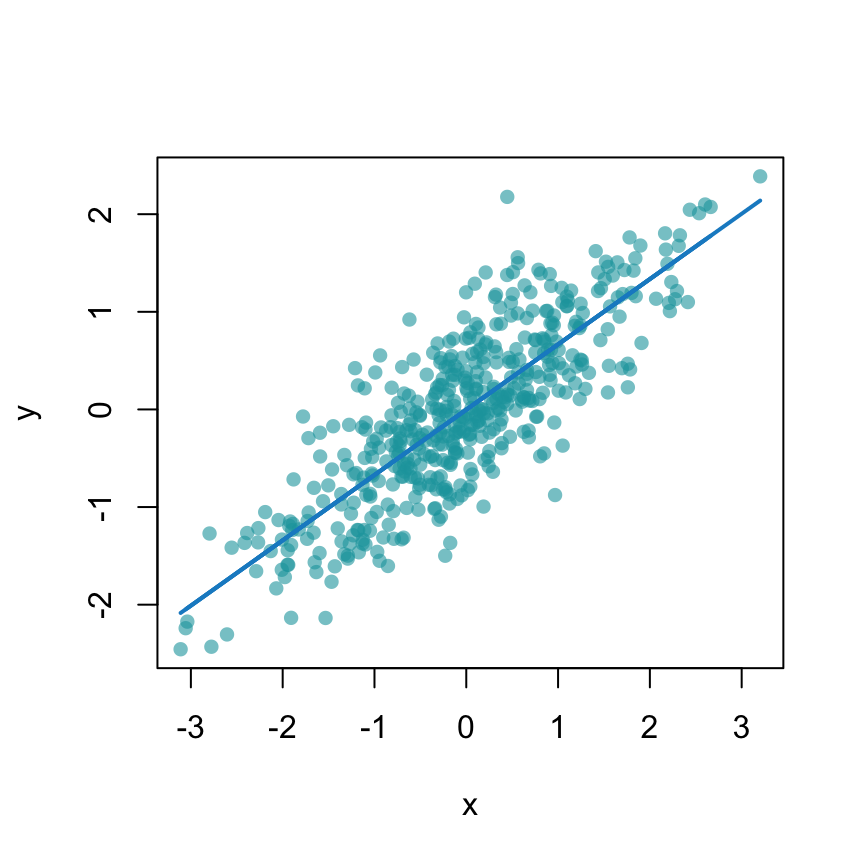
You use lines() to add a line on top of a scatterplot drawn with plot().lines() accepts x and y vectors of coordinates:
set.seed(2020)
x <- rnorm(500)
y <- 0.73 * x + 0.5 * rnorm(500)
xy.fit <- lm(y~x)$fitted
plot(x, y, pch = 16, col = "#18A3AC99")
lines(x, xy.fit, col = "#178CCB", lwd = 2)
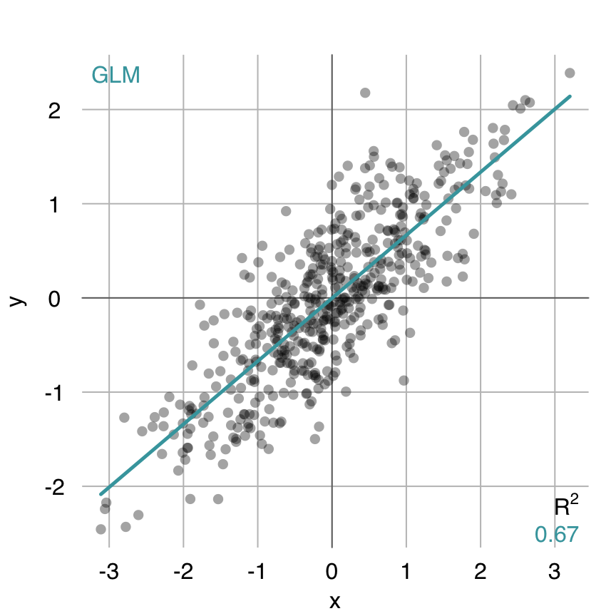
In rtemis, you can use argument fit to use any supported algorithm (see modSelect()) to estimate the fit:
mplot3_xy(x, y, fit = "glm")
49.1.7 Logistic Regression
For logistic regression, i.e. classification, you can use glm() with family = binomial
Using the same dataset, let’s predict diabetes status:
diabetes_mod <- glm(diabetes ~ ., data = PimaIndiansDiabetes2,
                    family = "binomial")
diabetes_mod
Call:  glm(formula = diabetes ~ ., family = "binomial", data = PimaIndiansDiabetes2)

Coefficients:
(Intercept)     pregnant      glucose     pressure      triceps      insulin
 -1.004e+01    8.216e-02    3.827e-02   -1.420e-03    1.122e-02   -8.253e-04
       mass     pedigree          age
  7.054e-02    1.141e+00    3.395e-02

Degrees of Freedom: 391 Total (i.e. Null);  383 Residual
  (376 observations deleted due to missingness)
Null Deviance:      498.1
Residual Deviance: 344 AIC: 362summary(diabetes_mod)
Call:
glm(formula = diabetes ~ ., family = "binomial", data = PimaIndiansDiabetes2)

Coefficients:
              Estimate Std. Error z value Pr(>|z|)
(Intercept) -1.004e+01  1.218e+00  -8.246  < 2e-16 ***
pregnant     8.216e-02  5.543e-02   1.482  0.13825
glucose      3.827e-02  5.768e-03   6.635 3.24e-11 ***
pressure    -1.420e-03  1.183e-02  -0.120  0.90446
triceps      1.122e-02  1.708e-02   0.657  0.51128
insulin     -8.253e-04  1.306e-03  -0.632  0.52757
mass         7.054e-02  2.734e-02   2.580  0.00989 **
pedigree     1.141e+00  4.274e-01   2.669  0.00760 **
age          3.395e-02  1.838e-02   1.847  0.06474 .
---
Signif. codes:  0 '***' 0.001 '**' 0.01 '*' 0.05 '.' 0.1 ' ' 1

(Dispersion parameter for binomial family taken to be 1)

    Null deviance: 498.10  on 391  degrees of freedom
Residual deviance: 344.02  on 383  degrees of freedom
  (376 observations deleted due to missingness)
AIC: 362.02

Number of Fisher Scoring iterations: 5
49.2 Mass-univariate analysis
There are many cases where we have a large number of predictors and, along with any other number of tests or models, we may want to regress our outcome of interest on each covariate, one at a time.
Let’s create some synthetic data with 1000 cases and 100 covariates
The outcome is generated using just 4 of those 100 covariates and has added noise.
set.seed(2020)
n_col <- 100
n_row <- 1000
x <- as.data.frame(lapply(seq(n_col), function(i) rnorm(n_row)),
                   col.names = paste0("Feature_", seq(n_col)))
dim(x)
[1] 1000 100y <- 0.7 + x[, 10] + 0.3 * x[, 20] + 1.3 * x[, 30] + x[, 50] + rnorm(500)Let’s fit a linear model regressing y on each column of x using lm:
[1] 100To extract p-values for each model, we must find where exactly to look.
Let’s look into the first model:
(ms1 <- summary(mod.xy.massuni$mod1))
Call:
lm(formula = y ~ x[, i])

Residuals:
    Min      1Q  Median      3Q     Max
-8.5402 -1.4881 -0.0618  1.4968  5.8152

Coefficients:
            Estimate Std. Error t value Pr(>|t|)
(Intercept)  0.61800    0.06878   8.985   <2e-16 ***
x[, i]       0.08346    0.06634   1.258    0.209
---
Signif. codes:  0 '***' 0.001 '**' 0.01 '*' 0.05 '.' 0.1 ' ' 1

Residual standard error: 2.174 on 998 degrees of freedom
Multiple R-squared:  0.001584,  Adjusted R-squared:  0.0005831
F-statistic: 1.583 on 1 and 998 DF, p-value: 0.2086ms1$coefficients Estimate Std. Error t value Pr(>|t|)
(Intercept) 0.61800326 0.06878142 8.985032 1.266204e-18
x[, i] 0.08346393 0.06634074 1.258110 2.086464e-01The p-values for each feature is stored in row 1, column 4 fo the coefficients matrix. Let’s extract all of them:
Let’s see which variable are significant at the 0.05:
which(mod.xy.massuni.pvals < 0.05) mod5 mod10 mod12 mod20 mod28 mod30 mod42 mod50 mod61 mod65 mod72 mod82 mod85
5 10 12 20 28 30 42 50 61 65 72 82 85
mod91 mod94 mod99
91 94 99 …and which are significant at the 0.01 level:
which(mod.xy.massuni.pvals < 0.01)mod10 mod20 mod28 mod30 mod50
10 20 28 30 50 49.3 Correction for multiple comparisons
We’ve performed a large number of tests and before reporting the results, we need to control for multiple comparisons.
To do that, we use R’s p.adjust() function. It adjusts a vector of p-values to account for multiple comparisons using one of multiple methods. The default, and recommended, is the Holm method. It ensures that FWER < α, i.e. controls the family-wise error rate, a.k.a. the probability of making one or more false discoveries (Type I errors)
mod.xy.massuni.pvals.holm_adjusted <- p.adjust(mod.xy.massuni.pvals)Now, let’s see which features’ p-values survive the magical 0.05 threshold:
which(mod.xy.massuni.pvals.holm_adjusted < 0.05)mod10 mod20 mod30 mod50
10 20 30 50 These are indeed the correct features (not surprisingly, still reassuringly).
