50 Benchmarking & Profiling

Benchmarking is the process of timing the execution of code for the purpose of comparison. For example, you can compare the execution time of a program in two different systems, e.g. a laptop and a high performance server. Another common case is to compare the performance of two different programs that produce the same output on the same computer.

Profiling refers to timing the different steps of a program to identify bottlenecks and potential targets for optimization.

50.1 `system.time()`: Time the execution of an expression

The base package’s system.time() function allows you to measure the execution time of an R expression.

system.time(rnorm(9999999))

   user  system elapsed 
  0.305   0.007   0.312

“elapsed” time is real time in seconds.

“user” and “system” are time used by the CPU on different types of tasks (see ?proc.time).

As always, you can pass any R expression within curly brackets:

x <- rnorm(9999)
system.time({
    for (i in 2:9999) {
      x[i]
      x[i] <- x[i]^3
    }
})

   user  system elapsed 
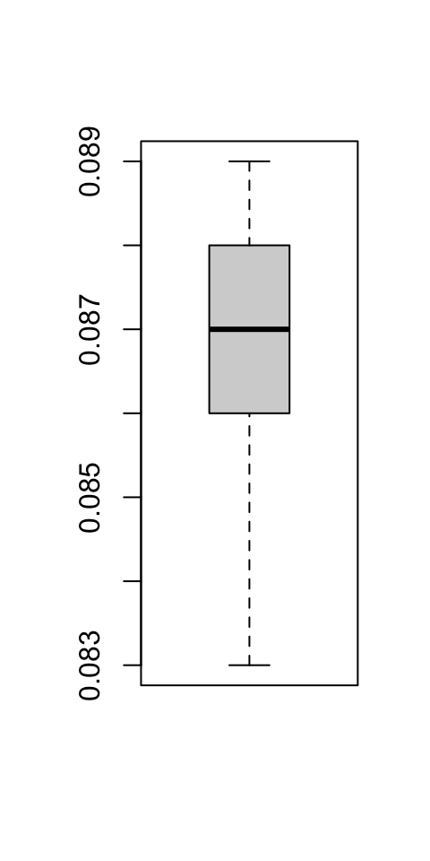
  0.002   0.000   0.002

You can use replicate() to get a measure of time over multiple executions and average it:

set.seed(2020)
x <- matrix(rnorm(500000), nrow = 5000)
y <- 12 + x[, 3] + x[, 5]^2 + x[, 7]^3 + rnorm(5000)
fit.glm <- function(x, y) glm.fit(x, y)
    
fit.glm_time10 <- replicate(10, system.time(fit.glm(x, y))[[1]])

boxplot(fit.glm_time10)

50.2 Compare execution times with `microbenchmark::microbenchmark()`

The microbenchmark package’s microbenchmark() function allows you to time the execution of multiple expressions with sub-millisecond accuracy. It will execute each command a number of times as defined by the times argument (default = 100), and output statistics of execution time per expression in nanoseconds. Using plot() on the output produces a boxplot comparing the time distributions.

# install.packages("microbenchmark")
library(microbenchmark)

50.2.1 Example: loop over matrix vs. data.frame

Let’s create xmat, a 500 by 5 matrix and, xdf a data.frame with the same data.

set.seed(2021)
xmat <- matrix(rnorm(500 * 5), nrow = 5)
xdf <- as.data.frame(xmat)

If you wanted to square either of them, you would just use ^2. Here, we create a function specifically to demonstrate the difference in working on a numeric matrix vs. a data.frame by using a nested loop that replaces each element one at a time.

silly_square <- function(x) {
  for (i in seq_len(NROW(x))) {
    for (j in seq_len(NCOL(x))) {
      x[i, j] <- x[i, j]^2
    }
  }
}

mat_df_sq <- microbenchmark(
  silly_square_mat = silly_square(xmat),
   silly_square_df = silly_square(xdf),
       mat_squared = xmat^2,
        df_squared = xdf^2
)

Warning in microbenchmark(silly_square_mat = silly_square(xmat),
silly_square_df = silly_square(xdf), : less accurate nanosecond times to avoid
potential integer overflows

class(mat_df_sq)

[1] "microbenchmark" "data.frame"

Print microbenchmark’s output:

mat_df_sq

Unit: microseconds
             expr       min         lq        mean    median         uq
 silly_square_mat   107.543   111.7865   135.07614   114.431   117.6905
  silly_square_df 40335.472 42334.3655 43649.35645 43320.272 44353.2875
      mat_squared     1.107     1.8655     3.05122     2.911     3.6900
       df_squared  9875.793 10685.0305 11735.24427 12122.388 12624.4945
       max neval
  2190.753   100
 71158.042   100
    15.990   100
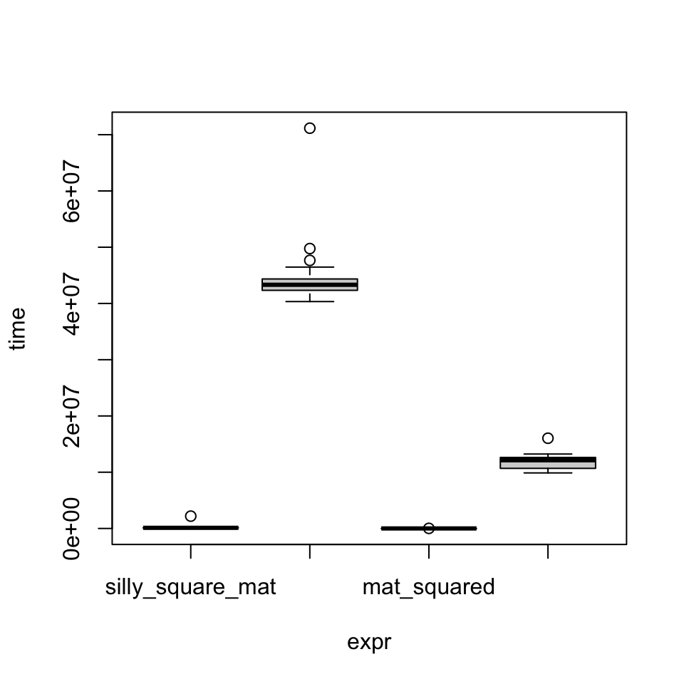
 16040.963   100

Notice how a) either operation is much faster on a matrix vs. a data.frame and b) vectorized squaring with ^2 is much faster than the nested loop as expected.

There is a plot() method for microbenchmark objects:

plot(mat_df_sq)

50.2.2 Example: Group means

Let’s perform a simple mean-by-group operation and compare three different approaches. As an example, we use the flights dataset from the nycflights13 package which includes data on 336,776 flights that departed from NY area airports in 2013. The data comes as a tibble, and we create data.frame and data.table versions.th

library(dplyr)
library(nycflights13)
library(data.table)
options(datatable.print.class = TRUE)

class(flights)

[1] "tbl_df"     "tbl"        "data.frame"

dim(flights)

[1] 336776     19

flights_df <- as.data.frame(flights)
flights_dt <- as.data.table(flights)

Compare performance of the same operation using different functions:

base R aggregate() with formula input
base R aggregate() with list input
base R tapply()

flights_aggregate_formula <- function() {
  aggregate(arr_delay ~ carrier, 
            data = flights_df,
            mean, na.rm = TRUE)
}
  
flights_aggregate <- function() {
  aggregate(flights_df$arr_delay, 
            by = list(flights_df$carrier), 
            mean, na.rm = TRUE)
}

flights_tapply <- function() {
  tapply(flights_df$arr_delay, 
         flights_df$carrier, 
         mean, na.rm = TRUE)
}

groupmean_3x <- microbenchmark(
  aggregate_formula = flights_aggregate_formula(),
          aggregate = flights_aggregate(),
             tapply = flights_tapply()
  )

groupmean_3x

Unit: milliseconds
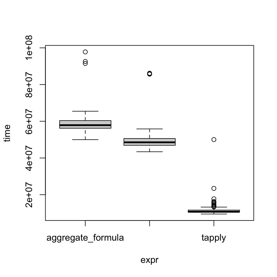
              expr       min       lq     mean   median       uq      max neval
 aggregate_formula 49.984125 56.19456 59.13615 57.88038 60.38195 97.78959   100
         aggregate 43.398500 46.89822 49.91139 48.52676 50.61108 86.17450   100
            tapply  9.478421 10.48790 11.85747 10.71896 11.61592 50.03513   100

plot(groupmean_3x)

50.3 Profile a function with `profvis()`

The profvis package’s profvis() function provides an interactive output to visualize the time spent in different calls within a program.

library(profvis)
profvis({
  hf <- read.csv("https://archive.ics.uci.edu/ml/machine-learning-databases/00519/heart_failure_clinical_records_dataset.csv")
  str(hf)
  lt5 <- which(sapply(hf, \(i) length(unique(i))) < 5)
  for (i in lt5) hf[, i] <- factor(hf[, i])
  index_numeric <- which(sapply(hf, is.numeric))
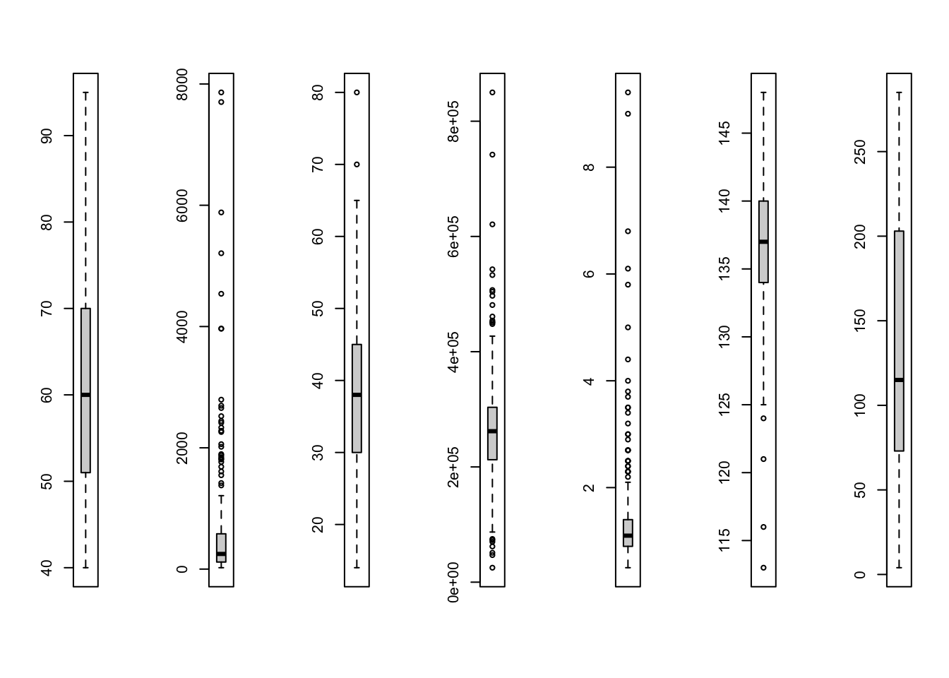
  par(mfrow = c(1, length(index_numeric)))
  for (i in index_numeric) boxplot(hf[, i])
  par(mfrow = c(1, 1))
})

'data.frame':   299 obs. of  13 variables:
 $ age                     : num  75 55 65 50 65 90 75 60 65 80 ...
 $ anaemia                 : int  0 0 0 1 1 1 1 1 0 1 ...
 $ creatinine_phosphokinase: int  582 7861 146 111 160 47 246 315 157 123 ...
 $ diabetes                : int  0 0 0 0 1 0 0 1 0 0 ...
 $ ejection_fraction       : int  20 38 20 20 20 40 15 60 65 35 ...
 $ high_blood_pressure     : int  1 0 0 0 0 1 0 0 0 1 ...
 $ platelets               : num  265000 263358 162000 210000 327000 ...
 $ serum_creatinine        : num  1.9 1.1 1.3 1.9 2.7 2.1 1.2 1.1 1.5 9.4 ...
 $ serum_sodium            : int  130 136 129 137 116 132 137 131 138 133 ...
 $ sex                     : int  1 1 1 1 0 1 1 1 0 1 ...
 $ smoking                 : int  0 0 1 0 0 1 0 1 0 1 ...
 $ time                    : int  4 6 7 7 8 8 10 10 10 10 ...
 $ DEATH_EVENT             : int  1 1 1 1 1 1 1 1 1 1 ...

50.1 system.time(): Time the execution of an expression

50.2 Compare execution times with microbenchmark::microbenchmark()

50.2.1 Example: loop over matrix vs. data.frame

50.2.2 Example: Group means

50.3 Profile a function with profvis()

50.1 `system.time()`: Time the execution of an expression

50.2 Compare execution times with `microbenchmark::microbenchmark()`

50.3 Profile a function with `profvis()`