35 data.table basics
35.1 data.table extends the functionality of the data.frame
Some of the ways in which a data.table differs from a data.frame:
- Many operations can be performed within a
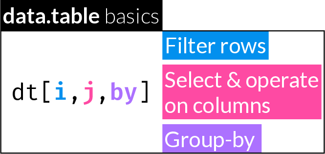
data.table’s “frame” (dt[i, j, by]): filter cases, select columns & operate on columns, group-by operations - Access column names directly without quoting
- Many operations can be performed “in-place” (i.e. with no assignment)
- Working on large datasets (e.g. millions of rows) can be orders of magnitude faster with a
data.tablethan adata.frame.
data.table operations remain as close as possible to data.frame operations, trying to extend rather than replace data.frame functionality.
data.table includes thorough and helpful error messages that often point to a solution. This includes common mistakes new users may make when trying commands that would work on a data.frame but not on a data.table.
35.1.1 Load the data.table package
35.2 Create a data.table
35.2.1 By assignment: data.table()
Let’s create a data.frame and a data.table to explore side by side.
df <- data.frame(A = 1:5,
                 B = c(1.2, 4.3, 9.7, 5.6, 8.1),
                 C = c("a", "b", "b", "a", "a"))
class(df)
[1] "data.frame"df A B C
1 1 1.2 a
2 2 4.3 b
3 3 9.7 b
4 4 5.6 a
5 5 8.1 adata.table() syntax is similar to data.frame() (differs in some arguments)
dt <- data.table(A = 1:5,
                 B = c(1.2, 4.3, 9.7, 5.6, 8.1),
                 C = c("a", "b", "b", "a", "a"))
class(dt)
[1] "data.table" "data.frame"dt A B C
<int> <num> <char>
1: 1 1.2 a
2: 2 4.3 b
3: 3 9.7 b
4: 4 5.6 a
5: 5 8.1 aNotice how a data.table object also inherits from data.frame. This means that if a method does not exist for data.table, the method for data.frame will be used (See classes and generic functions).
As part of improving efficiency, data.tables do away with row names. Instead of using row names, you should use a dedicated column or column with a row identifier/s (e.g. “ID”). this is advisable when working with data.frames as well.
A rather convenient option is to have data.tables print each column’s class below the column name. You can pass the argument class = TRUE to print() or set the global option datatable.print.class using options()
options(datatable.print.class = TRUE)
dt
A B C
<int> <num> <char>
1: 1 1.2 a
2: 2 4.3 b
3: 3 9.7 b
4: 4 5.6 a
5: 5 8.1 aSame as with a data.frame, to automatically convert strings to factors, you can use the stringsAsFactors argument:
dt2 <- data.table(A = 1:5,
                  B = c(1.2, 4.3, 9.7, 5.6, 8.1),
                  C = c("a", "b", "b", "a", "a"),
                  stringsAsFactors = TRUE)
dt2
A B C
<int> <num> <fctr>
1: 1 1.2 a
2: 2 4.3 b
3: 3 9.7 b
4: 4 5.6 a
5: 5 8.1 a
35.2.2 By coercion: as.data.table()
dat <- data.frame(A = 1:5,
                  B = c(1.2, 4.3, 9.7, 5.6, 8.1),
                  C = c("a", "b", "b", "a", "a"),
                  stringsAsFactors = TRUE)
dat
A B C
1 1 1.2 a
2 2 4.3 b
3 3 9.7 b
4 4 5.6 a
5 5 8.1 adat2 <- as.data.table(dat)
dat2 A B C
<int> <num> <fctr>
1: 1 1.2 a
2: 2 4.3 b
3: 3 9.7 b
4: 4 5.6 a
5: 5 8.1 a
35.2.3 By coercion in-place: setDT()
setDT() converts a list or data.frame into a data.table in-place. This means the object passed to setDT() is changed and you do not need to assign the output to a new object.
dat <- data.frame(A = 1:5,
                  B = c(1.2, 4.3, 9.7, 5.6, 8.1),
                  C = c("a", "b", "b", "a", "a"))
class(dat)
[1] "data.frame"You can similarly convert a data.table to a data.frame, in-place:
35.3 Display data.table structure with str()
str() works the same (and you should keep using it!)
str(df)'data.frame': 5 obs. of 3 variables:
$ A: int 1 2 3 4 5
$ B: num 1.2 4.3 9.7 5.6 8.1
$ C: chr "a" "b" "b" "a" ...str(dt)Classes 'data.table' and 'data.frame': 5 obs. of 3 variables:
$ A: int 1 2 3 4 5
$ B: num 1.2 4.3 9.7 5.6 8.1
$ C: chr "a" "b" "b" "a" ...
- attr(*, ".internal.selfref")=<externalptr>
35.4 Combine data.tables
cbind() and rbind() work on data.tables the same as on data.frames:
dt1 <- data.table(a = 1:5)
dt2 <- data.table(b = 11:15)
cbind(dt1, dt2)
a b
<int> <int>
1: 1 11
2: 2 12
3: 3 13
4: 4 14
5: 5 15rbind(dt1, dt1) a
<int>
1: 1
2: 2
3: 3
4: 4
5: 5
6: 1
7: 2
8: 3
9: 4
10: 535.5 Set column names in-place
dta <- data.table(
  ID = sample(8000:9000, size = 10),
  A = rnorm(10, mean = 47, sd = 8),
  W = rnorm(10, mean = 87, sd = 7)
)
dta
ID A W
<int> <num> <num>
1: 8683 65.38270 88.34494
2: 8831 51.19003 96.36451
3: 8333 63.82806 86.90661
4: 8044 52.50196 87.35874
5: 8760 38.77308 86.75976
6: 8973 41.92050 79.46510
7: 8873 54.94697 89.09996
8: 8089 60.04796 70.61579
9: 8259 48.08217 86.69053
10: 8181 59.72485 90.59614Use the syntax:
setnames(dt, old, new)
to change the column names of a data.table in-place.
Changes all column names:
    Patient_ID      Age   Weight
         <int>    <num>    <num>
 1:       8683 65.38270 88.34494
 2:       8831 51.19003 96.36451
 3:       8333 63.82806 86.90661
 4:       8044 52.50196 87.35874
 5:       8760 38.77308 86.75976
 6:       8973 41.92050 79.46510
 7:       8873 54.94697 89.09996
 8:       8089 60.04796 70.61579
 9:       8259 48.08217 86.69053
10:       8181 59.72485 90.59614
Change subset of names:
    Patient_ID Age_at_Admission Weight_at_Admission
         <int>            <num>               <num>
 1:       8683         65.38270            88.34494
 2:       8831         51.19003            96.36451
 3:       8333         63.82806            86.90661
 4:       8044         52.50196            87.35874
 5:       8760         38.77308            86.75976
 6:       8973         41.92050            79.46510
 7:       8873         54.94697            89.09996
 8:       8089         60.04796            70.61579
 9:       8259         48.08217            86.69053
10:       8181         59.72485            90.59614
old argument can also be integer index of column(s).
For example, change the name of the first column:
setnames(dta, 1, "Hospital_ID")
dta
Hospital_ID Age_at_Admission Weight_at_Admission
<int> <num> <num>
1: 8683 65.38270 88.34494
2: 8831 51.19003 96.36451
3: 8333 63.82806 86.90661
4: 8044 52.50196 87.35874
5: 8760 38.77308 86.75976
6: 8973 41.92050 79.46510
7: 8873 54.94697 89.09996
8: 8089 60.04796 70.61579
9: 8259 48.08217 86.69053
10: 8181 59.72485 90.5961435.6 Filter rows
There are many similarities and some notable differences in how indexing works in a data.table vs. a data.frame.
Filtering rows with an integer or logical index is largely the same in a data.frame and a data.table, but in a data.table you can omit the comma to select all columns:
df[c(1, 3, 5), ] A B C
1 1 1.2 a
3 3 9.7 b
5 5 8.1 adt[c(1, 3, 5), ] A B C
<int> <num> <char>
1: 1 1.2 a
2: 3 9.7 b
3: 5 8.1 adt[c(1, 3, 5)] A B C
<int> <num> <char>
1: 1 1.2 a
2: 3 9.7 b
3: 5 8.1 aUsing a variable that holds a row index, whether integer or logical:
rowid <- c(1, 3, 5)
df[rowid, ]
A B C
1 1 1.2 a
3 3 9.7 b
5 5 8.1 adt[rowid, ] A B C
<int> <num> <char>
1: 1 1.2 a
2: 3 9.7 b
3: 5 8.1 adt[rowid] A B C
<int> <num> <char>
1: 1 1.2 a
2: 3 9.7 b
3: 5 8.1 arowbn <- c(T, F, T, F, T)
df[rowbn, ] A B C
1 1 1.2 a
3 3 9.7 b
5 5 8.1 adt[rowbn, ] A B C
<int> <num> <char>
1: 1 1.2 a
2: 3 9.7 b
3: 5 8.1 adt[rowbn] A B C
<int> <num> <char>
1: 1 1.2 a
2: 3 9.7 b
3: 5 8.1 a35.6.1 Conditional filtering
As a reminder, there are a few ways to conditionally filter cases in a data.frame:
  A   B C
5 5 8.1 a A B C
5 5 8.1 a A B C
5 5 8.1 adata.table allows you to refer to column names directly and unquoted, which makes writing filter conditions easier/more compact:
The data.table package also includes an S3 method for subset() that works the same way as with a data.frame:
As another example, exclude cases based on missingness in a specific column:
adf <- as.data.frame(sapply(1:5, function(i) rnorm(10)))
adf |> head()
V1 V2 V3 V4 V5
1 0.902411777 1.2930875 1.0407948 1.0559136 0.5616985
2 0.580267346 -0.7832870 -0.6968492 1.2373361 1.6807925
3 -0.003170238 -1.0047477 0.7405467 -2.5859252 0.3343055
4 -0.922350665 -0.3273166 -1.1876403 0.4917402 1.7102410
5 0.739687336 -0.1770125 -0.9235757 -1.5588145 1.4051705
6 0.228370331 -1.2771214 -0.9437845 1.4142239 1.5548526adf[1, 3] <- adf[3, 4] <- adf[5, 3] <- adf[7, 3] <- NA
adt <- as.data.table(adf)adf[!is.na(adf$V3), ] V1 V2 V3 V4 V5
2 0.580267346 -0.7832870 -0.6968492 1.23733614 1.6807925
3 -0.003170238 -1.0047477 0.7405467 NA 0.3343055
4 -0.922350665 -0.3273166 -1.1876403 0.49174021 1.7102410
6 0.228370331 -1.2771214 -0.9437845 1.41422387 1.5548526
8 0.844595224 0.3321310 0.5219202 0.85338170 -2.2573230
9 0.019894582 0.6560011 0.9025611 -0.68491892 1.6959256
10 2.077229177 1.8165615 0.9781020 0.03906486 -2.2223410adt[!is.na(V3)] V1 V2 V3 V4 V5
<num> <num> <num> <num> <num>
1: 0.580267346 -0.7832870 -0.6968492 1.23733614 1.6807925
2: -0.003170238 -1.0047477 0.7405467 NA 0.3343055
3: -0.922350665 -0.3273166 -1.1876403 0.49174021 1.7102410
4: 0.228370331 -1.2771214 -0.9437845 1.41422387 1.5548526
5: 0.844595224 0.3321310 0.5219202 0.85338170 -2.2573230
6: 0.019894582 0.6560011 0.9025611 -0.68491892 1.6959256
7: 2.077229177 1.8165615 0.9781020 0.03906486 -2.222341035.7 Select columns
35.7.1 By position(s)
Selecting a single column in data.table does not drop to a vector, similar to using drop = FALSE in a data.frame:
df[, 1][1] 1 2 3 4 5df[, 1, drop = FALSE] A
1 1
2 2
3 3
4 4
5 5dt[, 1] A
<int>
1: 1
2: 2
3: 3
4: 4
5: 5Double bracket indexing of a single column works the same on a data.frame and a data.table, returning a vector:
df[[2]][1] 1.2 4.3 9.7 5.6 8.1dt[[2]][1] 1.2 4.3 9.7 5.6 8.1A vector of column positions returns a smaller data.table, similar to how it returns a smaller data.frame :
35.7.2 By name(s)
In data.table, you access column names directly without quoting or using the $ notation:
df[, "B"][1] 1.2 4.3 9.7 5.6 8.1df$B[1] 1.2 4.3 9.7 5.6 8.1dt[, B][1] 1.2 4.3 9.7 5.6 8.1Because of this, data.table requires a slightly different syntax to use a variable as a column index which can contain integer positions, logical index, or column names. While on a data.frame you can do pass an index vector directly:
  A   B
1 1 1.2
2 2 4.3
3 3 9.7
4 4 5.6
5 5 8.1df[, colbn] B C
1 1.2 a
2 4.3 b
3 9.7 b
4 5.6 a
5 8.1 adf[, colnm] A C
1 1 a
2 2 b
3 3 b
4 4 a
5 5 aTo do the same in a data.table, you must prefix the index vector with two dots:
dt[, ..colid] A B
<int> <num>
1: 1 1.2
2: 2 4.3
3: 3 9.7
4: 4 5.6
5: 5 8.1dt[, ..colbn] B C
<num> <char>
1: 1.2 a
2: 4.3 b
3: 9.7 b
4: 5.6 a
5: 8.1 adt[, ..colnm] A C
<int> <char>
1: 1 a
2: 2 b
3: 3 b
4: 4 a
5: 5 aThink of working inside the data.table frame (i.e. within the “[…]”) like an environment: you have direct access to the variables, i.e. columns within it. If you want to refer to variables outside the data.table, you must prefix their names with .. (similar to how you access the directory above your current working directory in the system shell).
Important
Always read error messages carefully, no matter what function or package you are using. In the case of data.table, the error messages are very informative and often point to the solution.
See what happens if you try to use the data.frame syntax by accident:
dt[, colid]Error in `[.data.table`(dt, , colid): j (the 2nd argument inside [...]) is a single symbol but column name 'colid' is not found. If you intended to select columns using a variable in calling scope, please try DT[, ..colid]. The .. prefix conveys one-level-up similar to a file system path.
Selecting a single column by name returns a vector:
dt[, A][1] 1 2 3 4 5Selecting one or more columns by name enclosed in list() or .() (which, in this case, is short for list()), always returns a data.table:
dt[, .(A)] A
<int>
1: 1
2: 2
3: 3
4: 4
5: 5dt[, .(A, B)] A B
<int> <num>
1: 1 1.2
2: 2 4.3
3: 3 9.7
4: 4 5.6
5: 5 8.1
35.7.3 .SD & .SDcols
.SDcols is a special symbol that can be used to select columns of a data.table as an alternative to j. It can accept a vector of integer positions or column names. .SD is another special symbol that can be used in j and refers to either the entire data.table, or the subset defined by .SDcols, if present. The following can be used to select columns:
dt[, .SD, .SDcols = colid] A B
<int> <num>
1: 1 1.2
2: 2 4.3
3: 3 9.7
4: 4 5.6
5: 5 8.1One of the main uses of .SD is shown below in combination with lapply().
35.8 Add new column in-place
Use := assignment to add a new column in the existing data.table.
dt[, AplusB := A + B]
dt
A B C AplusB
<int> <num> <char> <num>
1: 1 1.2 a 2.2
2: 2 4.3 b 6.3
3: 3 9.7 b 12.7
4: 4 5.6 a 9.6
5: 5 8.1 a 13.1Note how dt was modified even though we did not run dt <- dt[, AplusB := A + B]
35.9 Add multiple columns in-place
You can define multiple new column names using a character vector of new column names on the left of := and a list on the right.
We can use lapply() since it always returns a list:
       A     B      C AplusB AtimesB    AoverB      logA      logB
   <int> <num> <char>  <num>   <num>     <num>     <num>     <num>
1:     1   1.2      a    2.2     1.2 0.8333333 0.0000000 0.1823216
2:     2   4.3      b    6.3     8.6 0.4651163 0.6931472 1.4586150
3:     3   9.7      b   12.7    29.1 0.3092784 1.0986123 2.2721259
4:     4   5.6      a    9.6    22.4 0.7142857 1.3862944 1.7227666
5:     5   8.1      a   13.1    40.5 0.6172840 1.6094379 2.0918641
You can also use := in a little more awkward syntax:
dt[, `:=`(AminusB = A - B, AoverC = A / B)]
dt
A B C AplusB AtimesB AoverB logA logB AminusB
<int> <num> <char> <num> <num> <num> <num> <num> <num>
1: 1 1.2 a 2.2 1.2 0.8333333 0.0000000 0.1823216 -0.2
2: 2 4.3 b 6.3 8.6 0.4651163 0.6931472 1.4586150 -2.3
3: 3 9.7 b 12.7 29.1 0.3092784 1.0986123 2.2721259 -6.7
4: 4 5.6 a 9.6 22.4 0.7142857 1.3862944 1.7227666 -1.6
5: 5 8.1 a 13.1 40.5 0.6172840 1.6094379 2.0918641 -3.1
AoverC
<num>
1: 0.8333333
2: 0.4651163
3: 0.3092784
4: 0.7142857
5: 0.617284035.10 Convert column type
35.10.1 Assignment by reference with :=
Use any base R coercion function (as.*) to convert a column in-place using the := notation
dt[, A := as.numeric(A)]
dt
A B C AplusB AtimesB AoverB logA logB AminusB
<num> <num> <char> <num> <num> <num> <num> <num> <num>
1: 1 1.2 a 2.2 1.2 0.8333333 0.0000000 0.1823216 -0.2
2: 2 4.3 b 6.3 8.6 0.4651163 0.6931472 1.4586150 -2.3
3: 3 9.7 b 12.7 29.1 0.3092784 1.0986123 2.2721259 -6.7
4: 4 5.6 a 9.6 22.4 0.7142857 1.3862944 1.7227666 -1.6
5: 5 8.1 a 13.1 40.5 0.6172840 1.6094379 2.0918641 -3.1
AoverC
<num>
1: 0.8333333
2: 0.4651163
3: 0.3092784
4: 0.7142857
5: 0.6172840
35.10.2 Delete columns in-place with :=
To delete a column, use := to set it to NULL:
dt[, AoverB := NULL]
dt
A B C AplusB AtimesB logA logB AminusB AoverC
<num> <num> <char> <num> <num> <num> <num> <num> <num>
1: 1 1.2 a 2.2 1.2 0.0000000 0.1823216 -0.2 0.8333333
2: 2 4.3 b 6.3 8.6 0.6931472 1.4586150 -2.3 0.4651163
3: 3 9.7 b 12.7 29.1 1.0986123 2.2721259 -6.7 0.3092784
4: 4 5.6 a 9.6 22.4 1.3862944 1.7227666 -1.6 0.7142857
5: 5 8.1 a 13.1 40.5 1.6094379 2.0918641 -3.1 0.6172840Delete multiple columns
dt[, c("logA", "logB") := NULL]Or:
dt[, `:=`(AplusB = NULL, AminusB = NULL)]
dt
A B C AtimesB AoverC
<num> <num> <char> <num> <num>
1: 1 1.2 a 1.2 0.8333333
2: 2 4.3 b 8.6 0.4651163
3: 3 9.7 b 29.1 0.3092784
4: 4 5.6 a 22.4 0.7142857
5: 5 8.1 a 40.5 0.6172840
35.10.3 Fast loop-able assignment with set()
data.table’s set() is a loop-able version of the := operator. Use it in a for loop to operate on multiple columns.
Syntax: set(dt, i, j, value)
-
dtthe data.table to operate on -
ioptionally define which rows to operate on.i = NULLto operate on all rows -
jcolumn names or index to be assignedvalue -
valuevalues to be assigned tojby reference
As a simple example, transform the first two columns in-place by squaring:
for (i in 1:2) {
  set(dt, i = NULL, j = i, value = dt[[i]]^2)
}
35.11 Summarize
You can apply one or multiple summary functions on one or multiple columns. Surround the operations in list() or .() to output a new data.table holding the outputs of the operations, i.e. the input data.table remains unchanged.
   A_max A_min    A_sd
   <num> <num>   <num>
1:    25     1 9.66954
Example: Get the standard deviation of all numeric columns:
         A        B  AtimesB    AoverC
     <num>    <num>    <num>     <num>
1: 9.66954 37.35521 15.74462 0.2060219
If your function returns more than one value, the output will have multiple rows:
dt_range <- dt[, lapply(.SD, range), .SDcols = numid]
dt_range
A B AtimesB AoverC
<num> <num> <num> <num>
1: 1 1.44 1.2 0.3092784
2: 25 94.09 40.5 0.833333335.12 Set order
You can set the row order of a data.table in-place based on one or multiple columns’ values using setorder()
dt <- data.table(PatientID = sample(1001:9999, size = 10),
                 Height = rnorm(10, mean = 175, sd = 14),
                 Weight = rnorm(10, mean = 78, sd = 10),
                 Group = factor(sample(c("A", "B"), size = 10, replace = TRUE)))
dt
PatientID Height Weight Group
<int> <num> <num> <fctr>
1: 6771 173.7232 82.62411 A
2: 3090 191.7491 75.01137 B
3: 1234 195.2610 66.14451 B
4: 2111 152.4823 65.67971 B
5: 9473 173.5505 68.74644 B
6: 3894 154.0196 77.19524 A
7: 6942 183.7460 83.96044 A
8: 4712 165.1607 64.85735 A
9: 3430 184.5817 98.64208 B
10: 9606 170.3381 82.52088 BLet’s set the order by PatientID:
setorder(dt, PatientID)
dt
PatientID Height Weight Group
<int> <num> <num> <fctr>
1: 1234 195.2610 66.14451 B
2: 2111 152.4823 65.67971 B
3: 3090 191.7491 75.01137 B
4: 3430 184.5817 98.64208 B
5: 3894 154.0196 77.19524 A
6: 4712 165.1607 64.85735 A
7: 6771 173.7232 82.62411 A
8: 6942 183.7460 83.96044 A
9: 9473 173.5505 68.74644 B
10: 9606 170.3381 82.52088 BLet’s re-order, always in-place, by group and then by height:
setorder(dt, Group, Height)
dt
PatientID Height Weight Group
<int> <num> <num> <fctr>
1: 3894 154.0196 77.19524 A
2: 4712 165.1607 64.85735 A
3: 6771 173.7232 82.62411 A
4: 6942 183.7460 83.96044 A
5: 2111 152.4823 65.67971 B
6: 9606 170.3381 82.52088 B
7: 9473 173.5505 68.74644 B
8: 3430 184.5817 98.64208 B
9: 3090 191.7491 75.01137 B
10: 1234 195.2610 66.14451 B35.13 Group-by operations
Up to now, we have learned how to use the data.table frame dat[i, j] to filter cases in i or add/remove/transform columns in-place in j. dat[i, j, by] allows to perform operations separately on groups of cases.
dt <- data.table(A = 1:5,
                 B = c(1.2, 4.3, 9.7, 5.6, 8.1),
                 C = rnorm(5),
                 Group = c("a", "b", "b", "a", "a"))
dt
A B C Group
<int> <num> <num> <char>
1: 1 1.2 -1.7243334 a
2: 2 4.3 -0.8421823 b
3: 3 9.7 0.7892740 b
4: 4 5.6 0.2640193 a
5: 5 8.1 -0.1807966 a35.13.1 Group-by summary
As we’ve seen, using .() or list() in j, returns a new data.table:
35.13.2 Group-by operation and assignment
Making an assignment with := in j, adds a column in-place. If you combine such an assignment with a group-by operation, the same value will be assigned to all cases of the group:
dt[, mean_A_by_Group := mean(A), by = Group]
dt
A B C Group mean_A_by_Group
<int> <num> <num> <char> <num>
1: 1 1.2 -1.7243334 a 3.333333
2: 2 4.3 -0.8421823 b 2.500000
3: 3 9.7 0.7892740 b 2.500000
4: 4 5.6 0.2640193 a 3.333333
5: 5 8.1 -0.1807966 a 3.33333335.14 Apply functions to columns
Any function that returns a list can be used in j to return a new data.table - therefore lapply is perfect for getting summary on multiple columns. This is another example where you have to use the .SD notation:
dt1 <- as.data.table(sapply(1:3, \(i) rnorm(10)))
dt1
V1 V2 V3
<num> <num> <num>
1: -0.8596756 -0.3872235 -0.4501584
2: 0.1268567 -0.7755533 0.3603807
3: 0.7298289 -1.6452208 0.9137217
4: -0.5078484 0.3122644 -1.2696068
5: -0.9108845 -1.4404961 -0.5620521
6: 1.5740202 -2.1390065 1.4832881
7: -2.3917697 -0.3722932 -0.1926057
8: -0.6004372 -0.2706900 0.8909017
9: -0.2267385 0.5405553 1.0833964
10: -0.6378043 1.6665854 1.6748571 Alpha Beta Gamma
<num> <num> <num>
1: -0.3704452 -0.4511078 0.3932123You can specify which columns to operate on using the .SDcols argument:
dt2 <- data.table(A = 1:5,
                  B = c(1.2, 4.3, 9.7, 5.6, 8.1),
                  C = rnorm(5),
                  Group = c("a", "b", "b", "a", "a"))
dt2
A B C Group
<int> <num> <num> <char>
1: 1 1.2 -0.5960686 a
2: 2 4.3 1.4363967 b
3: 3 9.7 -0.5264020 b
4: 4 5.6 1.6849226 a
5: 5 8.1 0.5502497 adt2[, lapply(.SD, mean), .SDcols = 1:2] A B
<num> <num>
1: 3 5.78 A B
<num> <num>
1: 3 5.78 A B
<num> <num>
1: 3 5.78You can combine .SDcols and by:
    Group     B         C
   <char> <num>     <num>
1:      a   5.6 0.5502497
2:      b   7.0 0.4549973
Create multiple new columns from transformation of existing and store with custom prefix:
dt1 Alpha Beta Gamma
<num> <num> <num>
1: -0.8596756 -0.3872235 -0.4501584
2: 0.1268567 -0.7755533 0.3603807
3: 0.7298289 -1.6452208 0.9137217
4: -0.5078484 0.3122644 -1.2696068
5: -0.9108845 -1.4404961 -0.5620521
6: 1.5740202 -2.1390065 1.4832881
7: -2.3917697 -0.3722932 -0.1926057
8: -0.6004372 -0.2706900 0.8909017
9: -0.2267385 0.5405553 1.0833964
10: -0.6378043 1.6665854 1.6748571 Alpha Beta Gamma Alpha_abs Beta_abs Gamma_abs
<num> <num> <num> <num> <num> <num>
1: -0.8596756 -0.3872235 -0.4501584 0.8596756 0.3872235 0.4501584
2: 0.1268567 -0.7755533 0.3603807 0.1268567 0.7755533 0.3603807
3: 0.7298289 -1.6452208 0.9137217 0.7298289 1.6452208 0.9137217
4: -0.5078484 0.3122644 -1.2696068 0.5078484 0.3122644 1.2696068
5: -0.9108845 -1.4404961 -0.5620521 0.9108845 1.4404961 0.5620521
6: 1.5740202 -2.1390065 1.4832881 1.5740202 2.1390065 1.4832881
7: -2.3917697 -0.3722932 -0.1926057 2.3917697 0.3722932 0.1926057
8: -0.6004372 -0.2706900 0.8909017 0.6004372 0.2706900 0.8909017
9: -0.2267385 0.5405553 1.0833964 0.2267385 0.5405553 1.0833964
10: -0.6378043 1.6665854 1.6748571 0.6378043 1.6665854 1.6748571dt2 A B C Group
<int> <num> <num> <char>
1: 1 1.2 -0.5960686 a
2: 2 4.3 1.4363967 b
3: 3 9.7 -0.5264020 b
4: 4 5.6 1.6849226 a
5: 5 8.1 0.5502497 acols <- c("A", "C")
dt2[, paste0(cols, "_groupMean") := lapply(.SD, mean), .SDcols = cols, by = Group]
dt2 A B C Group A_groupMean C_groupMean
<int> <num> <num> <char> <num> <num>
1: 1 1.2 -0.5960686 a 3.333333 0.5463679
2: 2 4.3 1.4363967 b 2.500000 0.4549973
3: 3 9.7 -0.5264020 b 2.500000 0.4549973
4: 4 5.6 1.6849226 a 3.333333 0.5463679
5: 5 8.1 0.5502497 a 3.333333 0.546367935.15 Row-wise operations
dt <- data.table(a = 1:5, b = 11:15, c = 21:25,
                 d = 31:35, e = 41:45)
dt
a b c d e
<int> <int> <int> <int> <int>
1: 1 11 21 31 41
2: 2 12 22 32 42
3: 3 13 23 33 43
4: 4 14 24 34 44
5: 5 15 25 35 45To operate row-wise, we can use by = 1:nrow(dt). For example, to add a column, in-place, with row-wise sums of variables b through d:
35.16 Watch out for data.table error messages
For example