Bagging , i.e. bootstrap aggregating, is a core ML ensemble technique which can reduce bias and variance of a learner. In bagging, the training set is resampled, and a model is trained on each resample. Predictions from each model are averaged to give the final estimate. Random Forest is the most popular application of bagging. rtemis allows you to easily bag any learner - but don’t try bagging a linear model.
Regression
First, create some synthetic data:
set.seed (2018 )<- rnormmat (500 , 50 )colnames (x) <- paste0 ("Feature" , 1 : 50 )<- rnorm (50 )<- x[, 3 ] ^ 2 + x[, 10 ] * 2.3 + x[, 15 ] * .5 + x[, 20 ] * .7 + x[, 27 ] * 3.4 + x[, 31 ] * 1.2 + rnorm (500 )<- data.frame (x, y)<- resample (dat, seed = 2018 )01-07-24 00:31:43 Input contains more than one columns; will stratify on last [resample]
.: Resampling Parameters
n.resamples : 10
resampler : strat.sub
stratify.var : y
train.p : 0.75
strat.n.bins : 4
01-07-24 00:31:43 Created 10 stratified subsamples [resample]
<- dat[res$ Subsample_1, ]<- dat[- res$ Subsample_1, ]
Single CART
Let’s start by training a single CART of depth 3:
<- s_CART (dat.train, dat.test,maxdepth = 3 ,print.plot = FALSE )01-07-24 00:31:43 Hello, egenn [s_CART]
.: Regression Input Summary
Training features: 373 x 50
Training outcome: 373 x 1
Testing features: 127 x 50
Testing outcome: 127 x 1
01-07-24 00:31:43 Training CART... [s_CART]
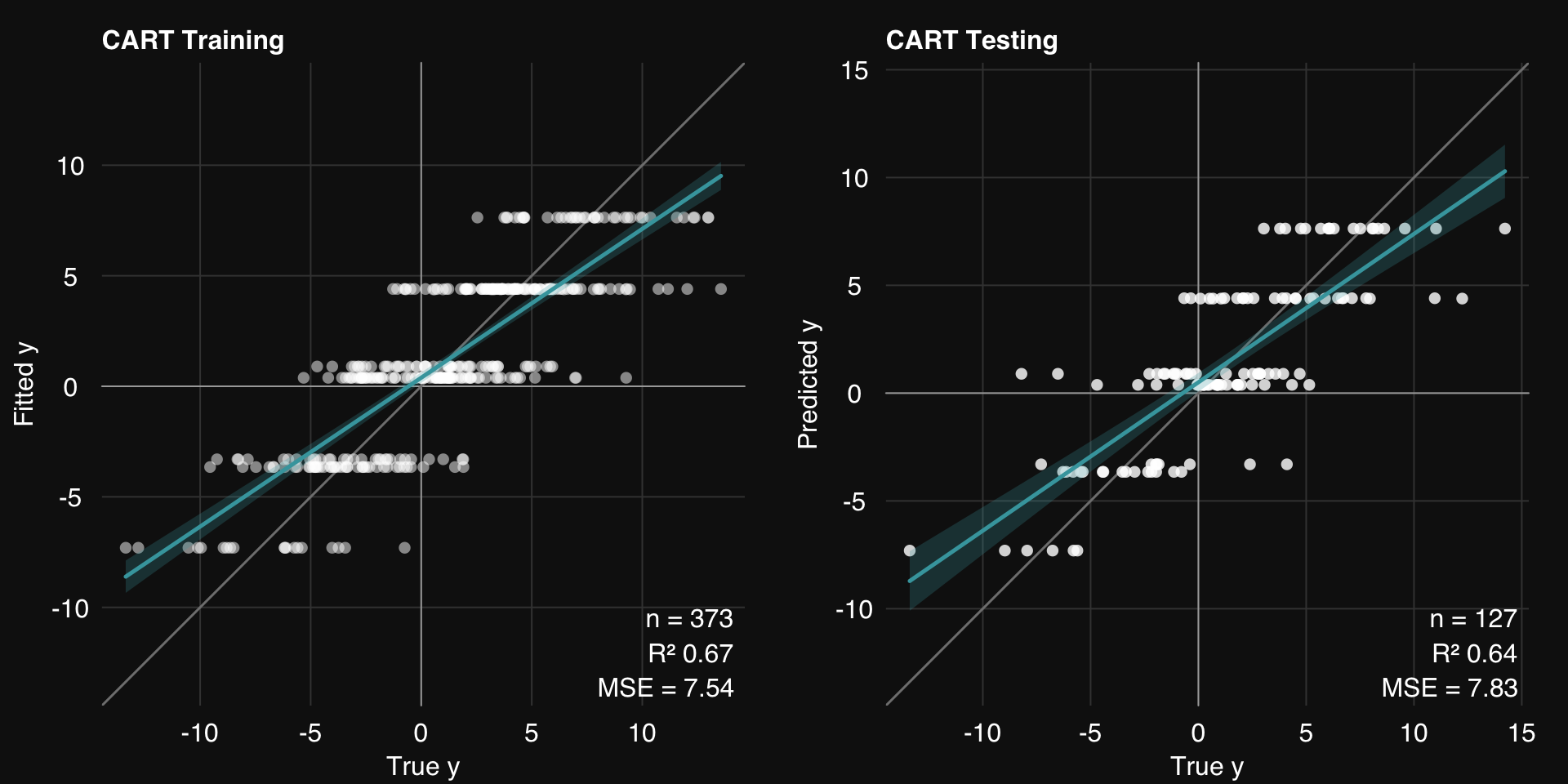
.: CART Regression Training Summary
MSE = 7.54 (67.32%)
RMSE = 2.75 (42.84%)
MAE = 2.17 (43.35%)
r = 0.82 (p = 3.9e-92)
R sq = 0.67
.: CART Regression Testing Summary
MSE = 7.83 (64.11%)
RMSE = 2.80 (40.09%)
MAE = 2.17 (40.52%)
r = 0.80 (p = 7.3e-30)
R sq = 0.64
01-07-24 00:31:43 Completed in 3.2e-04 minutes (Real: 0.02; User: 0.02; System: 1e-03) [s_CART]
rtlayout (1 , 2 )$ plotFitted ()$ plotPredicted ()
Bagged CARTs
Let’s bag 20 CARTs:
<- bag (dat.train, dat.test,mod = 'cart' , k = 20 ,mod.params = list (maxdepth = 3 ),.resample = setup.resample (resampler = "bootstrap" ,n.resamples = 20 ),print.plot = FALSE )01-07-24 00:31:43 Hello, egenn [bag]
.: Regression Input Summary
Training features: 373 x 50
Training outcome: 373 x 1
Testing features: 127 x 50
Testing outcome: 127 x 1
.: Parameters
mod : cart
mod.params :
maxdepth : 3
01-07-24 00:31:43 Bagging 20 Classification and Regression Trees... [bag]
01-07-24 00:31:43 Outer resampling: Future plan set to multicore with 8 workers [resLearn]
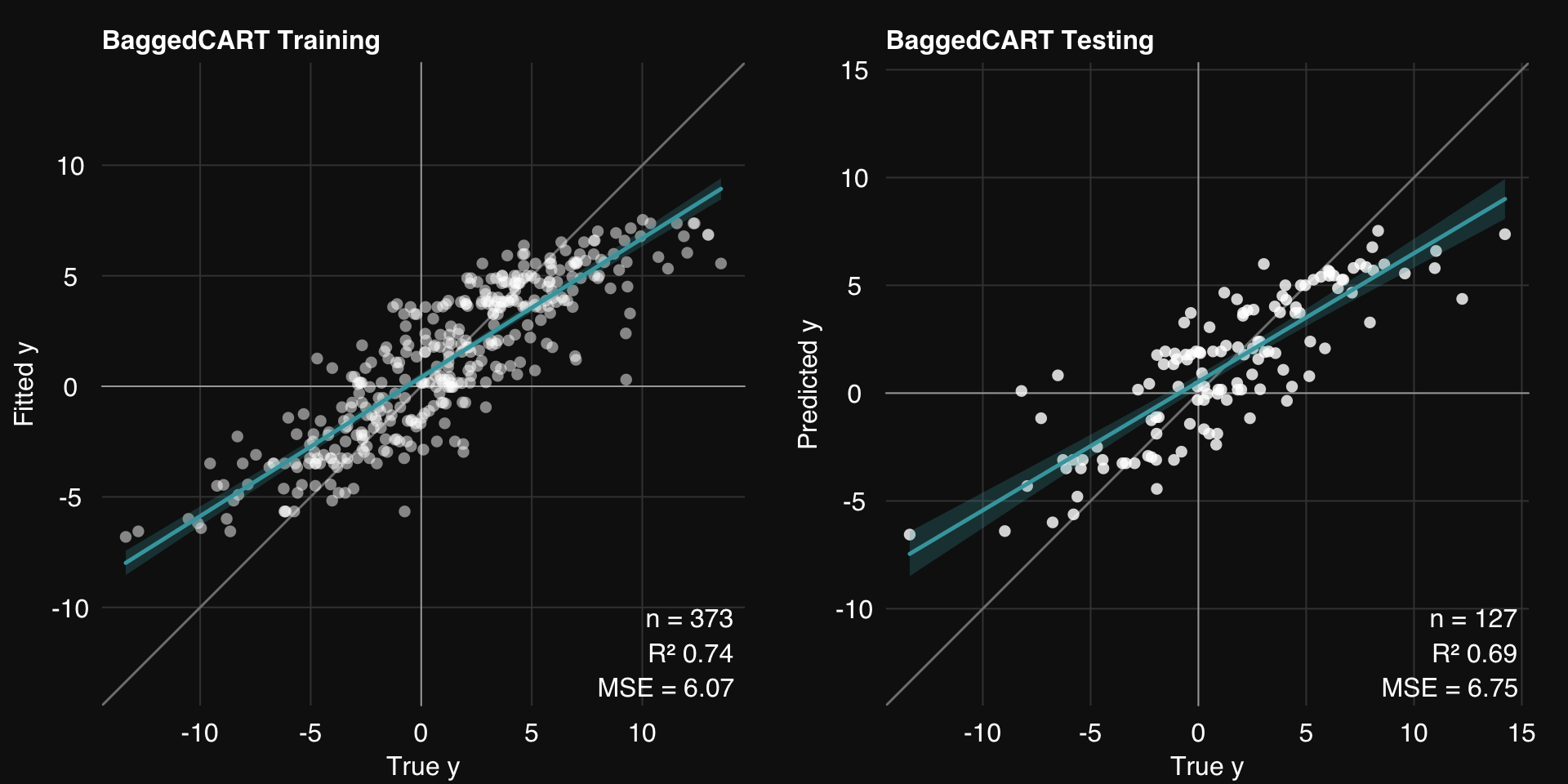
.: Regression Training Summary
MSE = 6.07 (73.72%)
RMSE = 2.46 (48.73%)
MAE = 1.92 (50.09%)
r = 0.87 (p = 5e-117)
R sq = 0.74
.: Regression Testing Summary
MSE = 6.75 (69.06%)
RMSE = 2.60 (44.38%)
MAE = 1.98 (45.56%)
r = 0.84 (p = 3e-35)
R sq = 0.69
01-07-24 00:31:44 Completed in 0.01 minutes (Real: 0.49; User: 0.14; System: 0.20) [bag]
rtlayout (1 , 2 )$ plotFitted ()$ plotPredicted ()
We make two important observations:
Both training and testing error is reduced
Generalizability is increased, i.e. the gap between training and testing error is decreased
Classification
We’ll use the Sonar dataset:
library (mlbench)data (Sonar)<- resample (Sonar)01-07-24 00:31:44 Input contains more than one columns; will stratify on last [resample]
.: Resampling Parameters
n.resamples : 10
resampler : strat.sub
stratify.var : y
train.p : 0.75
strat.n.bins : 4
01-07-24 00:31:44 Using max n bins possible = 2 [strat.sub]
01-07-24 00:31:44 Created 10 stratified subsamples [resample]
<- Sonar[res$ Subsample_1, ]<- Sonar[- res$ Subsample_1, ]
Single CART
<- s_CART (sonar.train, sonar.test,maxdepth = 10 ,print.plot = FALSE )01-07-24 00:31:44 Hello, egenn [s_CART]
01-07-24 00:31:44 Imbalanced classes: using Inverse Frequency Weighting [prepare_data]
.: Classification Input Summary
Training features: 155 x 60
Training outcome: 155 x 1
Testing features: 53 x 60
Testing outcome: 53 x 1
01-07-24 00:31:44 Training CART... [s_CART]
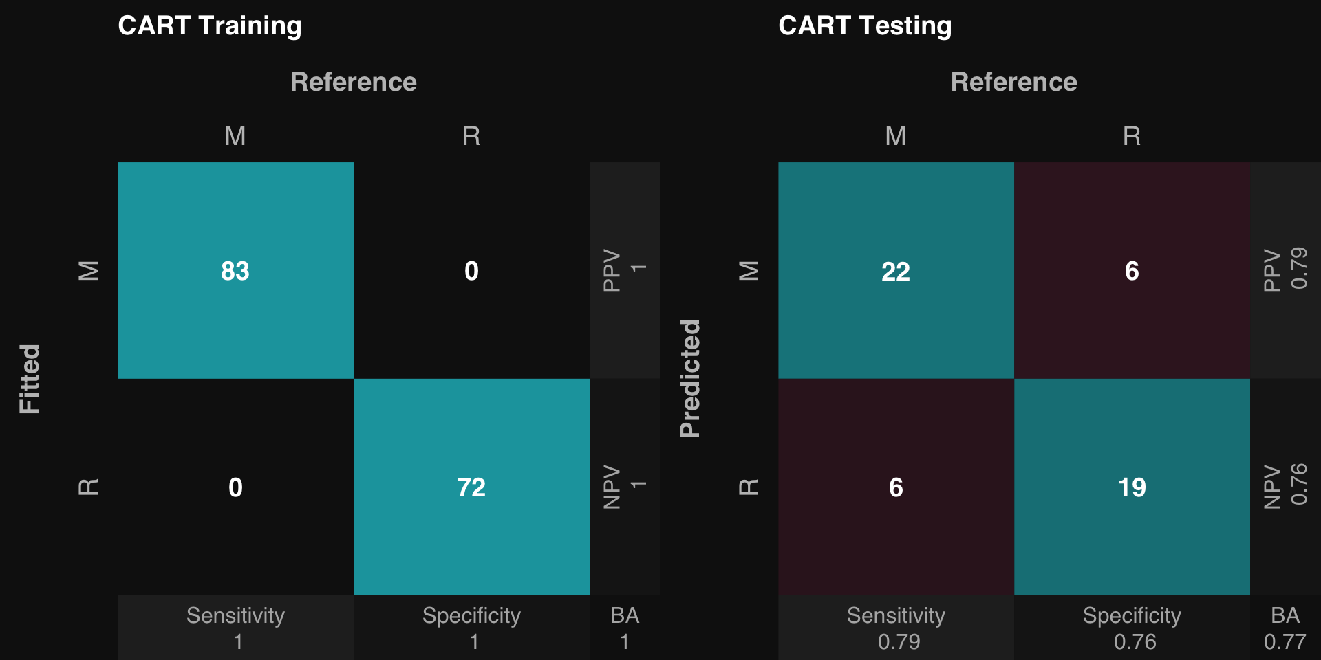
.: CART Classification Training Summary
Reference
Estimated M R
M 83 0
R 0 72
Overall
Sensitivity 1
Specificity 1
Balanced Accuracy 1
PPV 1
NPV 1
F1 1
Accuracy 1
AUC 1
Positive Class: M
.: CART Classification Testing Summary
Reference
Estimated M R
M 22 6
R 6 19
Overall
Sensitivity 0.7857
Specificity 0.7600
Balanced Accuracy 0.7729
PPV 0.7857
NPV 0.7600
F1 0.7857
Accuracy 0.7736
AUC 0.7729
Positive Class: M
01-07-24 00:31:45 Completed in 1.1e-03 minutes (Real: 0.07; User: 0.06; System: 0.01) [s_CART]
rtlayout (1 , 2 )$ plotFitted ()$ plotPredicted ()
Bagged CARTs
<- bag (sonar.train, sonar.test,mod = 'cart' , k = 20 ,mod.params = list (maxdepth = 10 ),.resample = setup.resample (resampler = "bootstrap" ,n.resamples = 20 ),print.plot = FALSE )01-07-24 00:31:45 Hello, egenn [bag]
01-07-24 00:31:45 Imbalanced classes: using Inverse Frequency Weighting [prepare_data]
.: Classification Input Summary
Training features: 155 x 60
Training outcome: 155 x 1
Testing features: 53 x 60
Testing outcome: 53 x 1
.: Parameters
mod : cart
mod.params :
maxdepth : 10
01-07-24 00:31:45 Bagging 20 Classification and Regression Trees... [bag]
01-07-24 00:31:45 Outer resampling: Future plan set to multicore with 8 workers [resLearn]
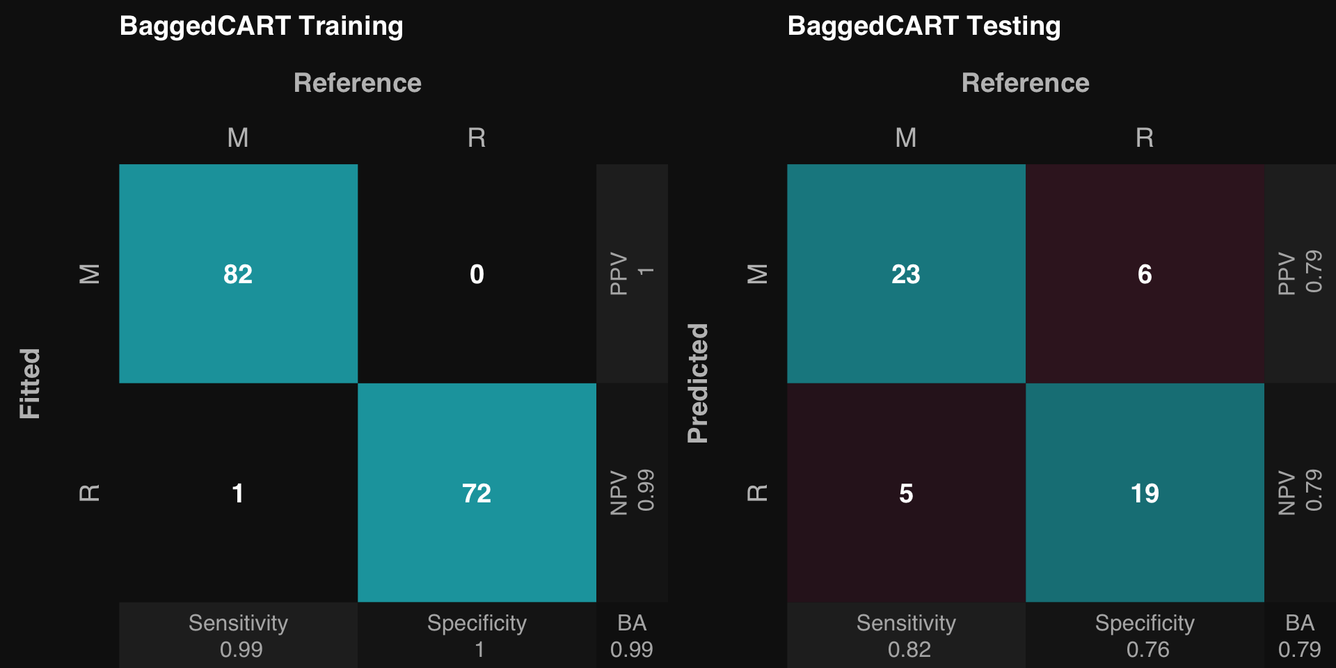
.: Classification Training Summary
Reference
Estimated M R
M 82 0
R 1 72
Overall
Sensitivity 0.9880
Specificity 1.0000
Balanced Accuracy 0.9940
PPV 1.0000
NPV 0.9863
F1 0.9939
Accuracy 0.9935
Positive Class: M
.: Classification Testing Summary
Reference
Estimated M R
M 23 6
R 5 19
Overall
Sensitivity 0.8214
Specificity 0.7600
Balanced Accuracy 0.7907
PPV 0.7931
NPV 0.7917
F1 0.8070
Accuracy 0.7925
Positive Class: M
01-07-24 00:31:45 Completed in 0.01 minutes (Real: 0.67; User: 0.19; System: 0.23) [bag]
rtlayout (1 , 2 )$ plotFitted ()$ plotPredicted ()


