data(Sonar, package = "mlbench")11 Automatic tuning & testing
rtemis supports a large number of algorithms for supervised learning. Individual functions to access each algorithm begin with s_. These function will output a single trained model and may, optionally, perform internal resampling of the training set to tune hyperparameters before training a final model on the full training set. You can get a full list of supported algorithms by running select_learn().
train is the main supervised learning function which performs nested resampling to tune hyperparameters (inner resampling) and assess generalizability (outer resampling) using any rtemis learner. All supervised learning functions (s_ functions and train) can accept either a feature matrix / data frame, x, and an outcome vector, y, separately, or a combined dataset x alone, in which case the last column should be the outcome.
For classification, the outcome should be a factor where the first level is the ‘positive’ case. For regression, the outcome should be numeric.
This vignette will walk through the analysis of an example dataset using train_cv().
Note: The train_cv() function replaces the original elevate() function.
11.1 Classification
Let’s use the sonar dataset, available in the mlbench package.
mod <- train_cv(Sonar)06-30-24 10:57:21 Hello, egenn [train_cv]
.:Classification Input Summary
Training features: 208 x 60
Training outcome: 208 x 1
06-30-24 10:57:21 Training Ranger Random Forest on 10 stratified subsamples... [train_cv]
06-30-24 10:57:21 Outer resampling plan set to sequential [resLearn]
.:Cross-validated Ranger
Mean Balanced Accuracy of 10 stratified subsamples: 0.83
06-30-24 10:57:22 Completed in 0.02 minutes (Real: 1.15; User: 2.20; System: 0.38) [train_cv]
By default, train uses random forest (using the ranger package which uses all available CPU threads) on 10 stratified subsamples to assess generalizability, with a 80% training - 20% testing split.
11.1.1 Plot confusion matrix
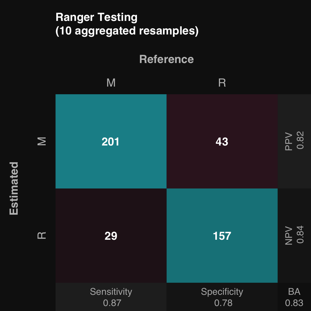
The output of train is an object that includes methods for plotting. $plot() plots the confusion matrix of all aggregated test sets
mod$plot()
It is really an alias for mod$plotPredicted(). The confusion matrix of the aggregated training sets can be plotted using mod$plotFitted().
11.1.2 Plot ROC
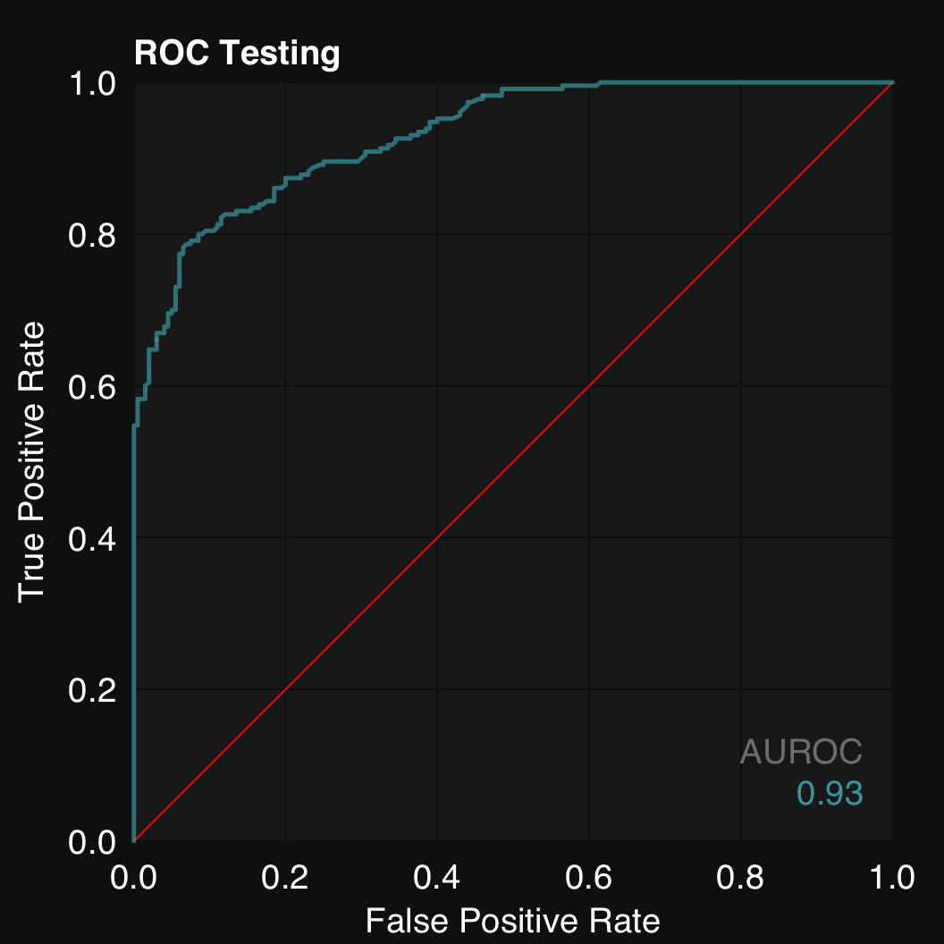
$plotROC()
mod$plotROC()
Similarly to mod$plot(), mod$plotROC() is an alias for mod$plotROCpredicted() and mod$plotROCfitted() is also available.
11.1.3 Plot variable importance
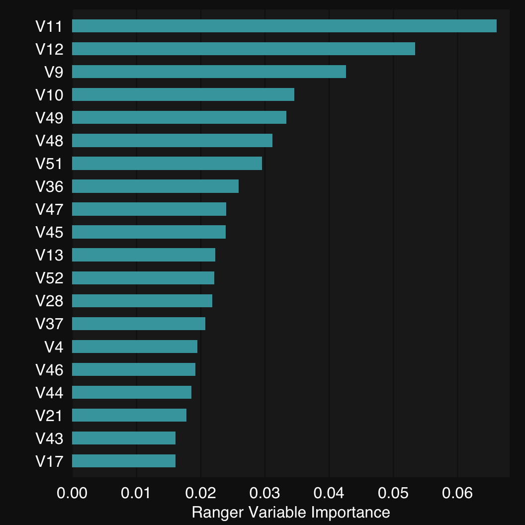
Finally, mod$plotVarImp() plots the variabple importance of the predictors. Use the plot.top argument to limit to this many top features.
mod$plotVarImp(plot.top = 20)
11.1.4 Describe
Each train object includes a very nifty describe() function:
mod$describe()Classification was performed using Ranger Random Forest. Model generalizability was assessed using 10 stratified subsamples. The mean Balanced Accuracy across all testing set resamples was 0.83.11.1.5 Resample performance
Field error.test.res is a list that holds the test-set error for each repeat.
Commonly, we use one repeat of multiple resamples (the default is 10 resamples, which is likely sufficient for bigger datasets. For smaller datasets it’s probably best to increase to 20 or 25).
11.1.5.1 Plot
You can use mplot3(), dplot3(), or other functions to visualize one (or multiple) resample performance metrics. For example:
dplot3_x(mod$error.test.res$CV_Ranger_repeat1$`Balanced Accuracy`,
xlab = "Balanced Accuracy")dplot3_box(mod$error.test.res$CV_Ranger_repeat1[, 1:8])11.1.5.2 Summary table
Mean, median, and SD of all metrics:
t(sapply(mod$error.test.res[[1]], function(i)
  data.frame(Mean = mean(i), Median = median(i), SD = sd(i))))
Mean Median SD
Sensitivity 0.873913 0.8695652 0.05957914
Specificity 0.785 0.8 0.0944281
Balanced Accuracy 0.8294565 0.8347826 0.04803547
PPV 0.828543 0.8356643 0.06170839
NPV 0.8479989 0.83125 0.06008998
F1 0.8483388 0.8444444 0.03975211
Accuracy 0.8325581 0.8372093 0.04625251
AUC 0.9313043 0.9304348 0.02715603
Brier Score 0.1281082 0.1319776 0.0157168
Log loss 0.4122931 0.4199908 0.0361969611.2 Regression
train_cv() for regression works just like in the above example for classification.
In the example below, we also show how to use check_data(), preprocess(), and decompose() as part of an analysis pipeline.
11.2.1 Create synthetic data
We create an input matrix of random numbers drawn from a normal distribution using rnormmat(), and a vector of random weights.
We matrix multiply the the input matrix with the weights and add some noise to create our output.
Finally, we replace some values with NA.
x <- rnormmat(400, 20)
w <- rnorm(20)
y <- x %*% w + rnorm(400)
x[sample(length(x), 30)] <- NA
11.2.2 Scenario 1: check_data - preprocess - train
11.2.2.1 Step 1: Check data with check_data
First step for every analysis should be to get some information on our data and perform some basic checks.
check_data(x) x: A data.table with 400 rows and 20 columns
Data types
* 20 numeric features
* 0 integer features
* 0 factors
* 0 character features
* 0 date features
Issues
* 0 constant features
* 0 duplicate cases
* 16 features include 'NA' values; 30 'NA' values total
* 16 numeric
Recommendations
* Consider imputing missing values or use complete cases only
11.2.2.2 Step 2: Preprocess data with preprocess
x <- preprocess(x, impute = TRUE)06-30-24 10:57:23 Hello, egenn [preprocess]
06-30-24 10:57:23 Imputing missing values using predictive mean matching with missRanger... [preprocess]
Missing value imputation by random forests
Variables to impute: V1, V3, V4, V6, V8, V9, V10, V11, V12, V13, V14, V15, V16, V17, V19, V20
Variables used to impute: V1, V2, V3, V4, V5, V6, V7, V8, V9, V10, V11, V12, V13, V14, V15, V16, V17, V18, V19, V20
iter 1
|
| | 0%
|
|==== | 6%
|
|========= | 12%
|
|============= | 19%
|
|================== | 25%
|
|====================== | 31%
|
|========================== | 38%
|
|=============================== | 44%
|
|=================================== | 50%
|
|======================================= | 56%
|
|============================================ | 62%
|
|================================================ | 69%
|
|==================================================== | 75%
|
|========================================================= | 81%
|
|============================================================= | 88%
|
|================================================================== | 94%
|
|======================================================================| 100%
06-30-24 10:57:23 Completed in 0.01 minutes (Real: 0.56; User: 2.84; System: 0.12) [preprocess]
Check the data again:
check_data(x) x: A data.table with 400 rows and 20 columns
Data types
* 20 numeric features
* 0 integer features
* 0 factors
* 0 character features
* 0 date features
Issues
* 0 constant features
* 0 duplicate cases
* 0 missing values
Recommendations
* Everything looks good
11.2.2.3 3. Train and test a model using 10 stratified subsamples
mod <- train_cv(x, y, alg = 'mars')06-30-24 10:57:23 Hello, egenn [train_cv]
.:Regression Input Summary
Training features: 400 x 20
Training outcome: 400 x 1
06-30-24 10:57:23 Training Multivariate Adaptive Regression Splines on 10 stratified subsamples... [train_cv]
06-30-24 10:57:23 Outer resampling plan set to sequential [resLearn]
.:Cross-validated MARS
Mean MSE of 10 stratified subsamples: 1.99
Mean MSE reduction: 87.70%
06-30-24 10:57:24 Completed in 0.02 minutes (Real: 1.10; User: 1.03; System: 0.04) [train_cv]
11.2.2.4 4. Plot true vs predicted
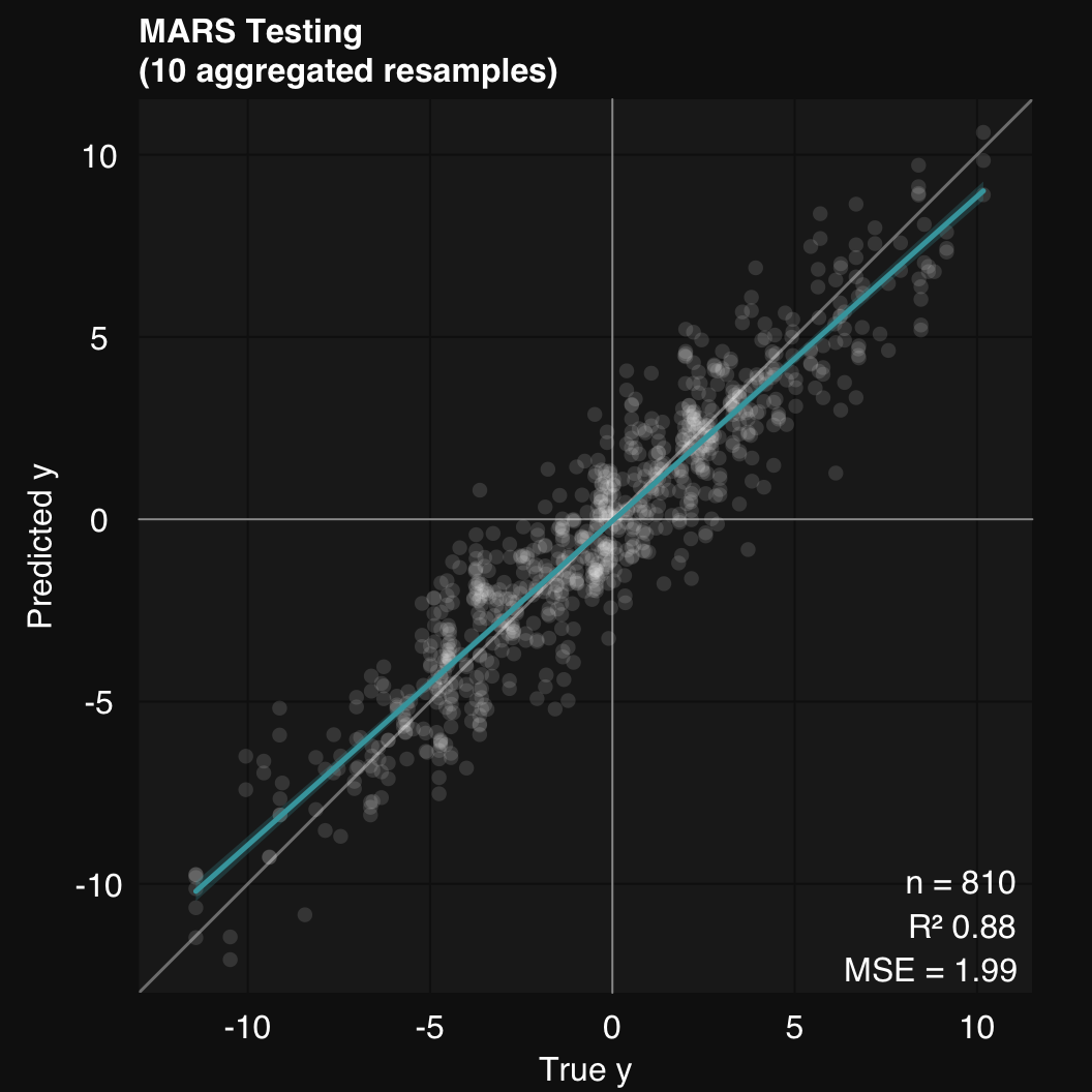
mod$plot()
11.2.2.5 Describe
mod$describe()Regression was performed using Multivariate Adaptive Regression Splines. Model generalizability was assessed using 10 stratified subsamples. The mean R-squared across all testing set resamples was 0.88.11.2.3 Resample performance
11.2.3.1 Plot
You can use mplot3(), dplot3(), or other functions to visualize one (or multiple) resample performance metrics. For example:
dplot3_x(mod$error.test.res$CV_MARS_repeat1$Rsq,
xlab = "R<sup>2</sup>")dplot3_box(mod$error.test.res$CV_MARS_repeat1[, 1:3])11.2.3.2 Summary table
Mean, median, and SD of all metrics:
t(sapply(mod$error.test.res[[1]][, c("MAE", "MSE", "RMSE", "Rsq")],
         function(i)
  data.frame(Mean = mean(i),
             Median = median(i),
             SD = sd(i))))
Mean Median SD
MAE 1.119013 1.076267 0.2946414
MSE 1.992201 1.757243 1.064494
RMSE 1.380328 1.325588 0.3107282
Rsq 0.8779902 0.8982814 0.0672326711.2.4 Scenario 2: train + preprocess
train_cv() allows you to automatically run preprocess() on a dataset using
the .preprocess argument.
In rtemis, arguments that add an extra step to the pipeline begin with a dot. train_cv()’s .preprocess accepts the same arguments as the preprocess() function.
For cases like this, rtemis provides helper functions which provide autocomplete functionality so as to avoid having to look up the original function’s usage (in this case, preprocess()).
We create a synthetic data set and combine x and y to show how train_cv() can work directly on a single data frame where the last column is the output. For this example, we use projection pursuit regression.
x <- rnormmat(400, 10, seed = 2018)
w <- rnorm(10)
y <- x %*% w + rnorm(400)
x[sample(length(x), 25)] <- NA
dat <- data.frame(x, y)
mod <- train_cv(dat, alg = 'ppr',
.preprocess = setup.preprocess(impute = TRUE))06-30-24 10:57:25 Hello, egenn [train_cv]
.:Regression Input Summary
Training features: 400 x 10
Training outcome: 400 x 1
06-30-24 10:57:25 Training Projection Pursuit Regression on 10 stratified subsamples... [train_cv]
06-30-24 10:57:25 Outer resampling plan set to sequential [resLearn]
.:Cross-validated PPR
Mean MSE of 10 stratified subsamples: 1.23
Mean MSE reduction: 88.07%
06-30-24 10:57:27 Completed in 0.04 minutes (Real: 2.55; User: 9.82; System: 1.09) [train_cv]
Notice that each message includes the date and time, followed by the name of the function being executed.
For example, above, note how preprocess.default() comes in to perform data imputation before model training.
preprocess.default() signifies it is working on an object of class data.frame. There is also a similar preprocess.data.table() that works on data.table objects.
mod$describe()Regression was performed using Projection Pursuit Regression. Data was preprocessed by imputing missing values using missRanger. Model generalizability was assessed using 10 stratified subsamples. The mean R-squared across all testing set resamples was 0.88.11.2.5 Scenario 3: train + decompose
train_cv() can also decompose a dataset ahead of modeling. We can direct train_cv() to perform decomposition ahead of modeling using the .decompose argument.
x <- rnormmat(400, 200)
w <- rnorm(200)
y <- x %*% w + rnorm(400)
dat <- data.frame(x, y)
mod <- train_cv(dat, 'glm', .decompose = setup.decompose(decom = "PCA", k = 10))
06-30-24 10:57:27 Hello, egenn [train_cv]
.:Regression Input Summary
Training features: 400 x 200
Training outcome: 400 x 1
06-30-24 10:57:27 Hello, egenn [d_PCA]
06-30-24 10:57:27 ||| Input has dimensions 400 rows by 200 columns, [d_PCA]
06-30-24 10:57:27 interpreted as 400 cases with 200 features. [d_PCA]
06-30-24 10:57:27 Performing Principal Component Analysis... [d_PCA]
06-30-24 10:57:27 Completed in 1.2e-03 minutes (Real: 0.07; User: 0.07; System: 1e-03) [d_PCA]
.:Regression Input Summary
Training features: 400 x 10
Training outcome: 400 x 1
06-30-24 10:57:27 Training Ranger Random Forest on 10 stratified subsamples... [train_cv]
06-30-24 10:57:27 Outer resampling plan set to sequential [resLearn]
.:Cross-validated Ranger
Mean MSE of 10 stratified subsamples: 204.91
Mean MSE reduction: 1.37%
06-30-24 10:57:28 Completed in 0.02 minutes (Real: 0.98; User: 3.43; System: 0.29) [train_cv]
mod$describe()Regression was performed using Ranger Random Forest. Input was projected to 10 dimensions using Principal Component Analysis. Model generalizability was assessed using 10 stratified subsamples. The mean R-squared across all testing set resamples was 0.02.